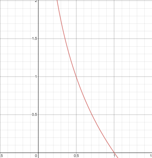
인코딩시 확률이 낮은 것들은 길게 코딩하고 높은 것들은 짧게 코딩한다.
\begin{align} E = {1/2} {\sum}_k{(y_k - t_k)^2} \end{align}
1
2
def SSE(y, t):
    return 0.5 * np.sum((y - t) ** 2)
1
2
3
4
5
6
7
8
9
10
11
# t = 정답 레이블
t = np.array([0, 0, 1, 0, 0, 0, 0, 0, 0, 0])

# y = softmax함수의 출력
y = np.array([0.1, 0.05, 0.6, 0.0, 0.05, 0.1, 0.0, 0.1, 0.0, 0.0])

# y2 = softmax함수의 출력
y2 = np.array([0.1, 0.05, 0.1, 0.0, 0.05, 0.1, 0.6, 0.3, 0.0, 0.0])

SSE(y, t)  # 0.09750000000000003
SSE(y2, t) # 0.6425
인코딩시 확률이 낮은 것들은 길게 코딩하고 높은 것들은 짧게 코딩한다.
\begin{align} -\log_2{P_i} \end{align}
\begin{align} E = {\sum}_i {p_i (-\log_2 P_i)} \end{align}
\begin{align} E = {\sum}_i{p_i(-log_2 Q_i)} \end{align}
1
2
3
def CEE(y, t):
    delta = 1e-7
    return -np.sum(t * np.log(y + delta))
1
2
3
4
5
6
7
8
9
10
11
# t = 정답 레이블
t = np.array([0, 0, 1, 0, 0, 0, 0, 0, 0, 0])

# y = softmax함수의 출력
y = np.array([0.1, 0.05, 0.6, 0.0, 0.05, 0.1, 0.0, 0.1, 0.0, 0.0])

# y2 = softmax함수의 출력
y2 = np.array([0.1, 0.05, 0.1, 0.0, 0.05, 0.1, 0.6, 0.3, 0.0, 0.0])

CEE(y, t)  # 0.510825457099338
CEE(y2, t) # 2.302584092994546
\begin{align} KL(p||q) = -{\sum}_i {p_i \log({q_i / p_i})} \end{align}
미니 배치
훈련 데이터 중 일부를 무작위로 가져온다. 가져온 미니배치의 손실 함수 값을 줄이는것이 목표이다.
기울기 산출
미니배치의 손실 함수 값을 줄이기 위해 각 가중치 매개변수의 기울기를 구한다. 기울기는 손실 함수의 값을 가장 작게 하는 방향을 제시한다.
매개변수 갱신
가중치 매개변수를 기울기 방향으로 조금씩 갱신한다.
1~3을 반복한다.
1
2
3
4
5
6
7
8
9
10
11
12
13
14
15
16
17
18
19
20
21
22
23
24
25
26
27
28
29
30
31
32
33
34
35
36
37
38
39
40
41
42
43
44
45
46
47
48
49
50
51
52
53
54
55
56
57
58
59
60
61
62
63
64
65
66
import sys, os

sys.path.append(os.pardir)  # 부모 디렉터리의 파일을 가져올 수 있도록 설정
from common.functions import *
from common.gradient import numerical_gradient

class TwoLayerNet:

    def __init__(self, input_size, hidden_size, output_size, weight_init_std=0.01):
        # 가중치 초기화
        self.params = {}
        self.params['W1'] = weight_init_std * np.random.randn(input_size, hidden_size)
        self.params['b1'] = np.zeros(hidden_size)
        self.params['W2'] = weight_init_std * np.random.randn(hidden_size, output_size)
        self.params['b2'] = np.zeros(output_size)

    def predict(self, x):
        W1, W2 = self.params['W1'], self.params['W2']
        b1, b2 = self.params['b1'], self.params['b2']

        a1 = np.dot(x, W1) + b1
        z1 = sigmoid(a1)
        a2 = np.dot(z1, W2) + b2
        y = softmax(a2)

        return y

    # x : 입력 데이터, t : 정답 레이블
    def loss(self, x, t):
        y = self.predict(x)

        return cross_entropy_error(y, t)

    def accuracy(self, x, t):
        y = self.predict(x)
        y = np.argmax(y, axis=1)
        t = np.argmax(t, axis=1)

        accuracy = np.sum(y == t) / float(x.shape[0])
        return accuracy

    # x : 입력 데이터, t : 정답 레이블
    def gradient(self, x, t):
        W1, W2 = self.params['W1'], self.params['W2']
        b1, b2 = self.params['b1'], self.params['b2']
        grads = {}

        batch_num = x.shape[0]

        # forward
        a1 = np.dot(x, W1) + b1
        z1 = sigmoid(a1)
        a2 = np.dot(z1, W2) + b2
        y = softmax(a2)

        # backward
        dy = (y - t) / batch_num
        grads['W2'] = np.dot(z1.T, dy)
        grads['b2'] = np.sum(dy, axis=0)

        da1 = np.dot(dy, W2.T)
        dz1 = sigmoid_grad(a1) * da1
        grads['W1'] = np.dot(x.T, dz1)
        grads['b1'] = np.sum(dz1, axis=0)

        return grads
1
2
3
4
5
6
7
8
9
10
11
12
13
14
15
16
17
18
19
20
21
22
23
24
25
26
27
28
29
30
31
32
33
34
35
36
37
38
39
40
41
42
43
44
45
46
47
48
49
50
51
52
import sys, os
# 부모 디렉터리의 파일을 가져올 수 있도록 설정
sys.path.append(os.pardir)
import numpy as np
import matplotlib.pyplot as plt
from dataset.mnist import load_mnist
from two_layer_net import TwoLayerNet
# 데이터 읽기
(x_train, t_train), (x_test, t_test) = load_mnist(normalize=True, one_hot_label=True)
network = TwoLayerNet(input_size=784, hidden_size=50, output_size=10)
# 하이퍼파라미터
iters_num = 10000 # 반복 횟수를 적절히 설정한다.
train_size = x_train.shape[0]
batch_size = 100 # 미니배치 크기
learning_rate = 0.1
train_loss_list = []
train_acc_list = []
test_acc_list = []
# 1에폭당 반복 수
iter_per_epoch = max(train_size / batch_size, 1)
for i in range(iters_num):
# 미니배치 획득
batch_mask = np.random.choice(train_size, batch_size)
x_batch = x_train[batch_mask]
t_batch = t_train[batch_mask]
# 기울기 계산
# grad = network.numerical_gradient(x_batch, t_batch)
grad = network.gradient(x_batch, t_batch)
# 매개변수 갱신
for key in ('W1', 'b1', 'W2', 'b2'):
network.params[key] -= learning_rate * grad[key]
# 학습 경과 기록
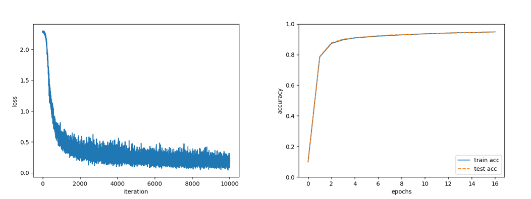
loss = network.loss(x_batch, t_batch)
train_loss_list.append(loss)
# 1에폭당 정확도 계산
if i % iter_per_epoch == 0:
train_acc = network.accuracy(x_train, t_train)
test_acc = network.accuracy(x_test, t_test)
train_acc_list.append(train_acc)
test_acc_list.append(test_acc)
print("train acc, test acc | " + str(train_acc) + ", " + str(test_acc))
코드: 밑바닥부터 시작하는 딥러닝
YouTube: 혁펜하임